Price elasticity of demand
Price elasticity of demand (PED or Ed) is a measure used in economics to show the responsiveness, or elasticity, of the quantity demanded of a good or service to a change in its price. More precisely, it gives the percentage change in quantity demanded in response to a one percent change in price (holding constant all the other determinants of demand, such as income). It was devised by Alfred Marshall.
Price elasticities are almost always negative, although analysts tend to ignore the sign even though this can lead to ambiguity. Only goods which do not conform to the law of demand, such as Veblen and Giffen goods, have a positive PED. In general, the demand for a good is said to be inelastic (or relatively inelastic) when the PED is less than one (in absolute value): that is, changes in price have a relatively small effect on the quantity of the good demanded. The demand for a good is said to be elastic (or relatively elastic) when its PED is greater than one (in absolute value): that is, changes in price have a relatively large effect on the quantity of a good demanded.
Revenue is maximised when price is set so that the PED is exactly one. The PED of a good can also be used to predict the incidence (or "burden") of a tax on that good. Various research methods are used to determine price elasticity, including test markets, analysis of historical sales data and conjoint analysis.
Contents |
Definition
PED is a measure of responsiveness of the quantity of a good or service demanded to changes in its price.[1] The formula for the coefficient of price elasticity of demand for a good is:[2][3][4]
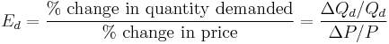
The above formula usually yields a negative value, due to the inverse nature of the relationship between price and quantity demanded, as described by the "law of demand".[3] For example, if the price increases by 5% and quantity demanded decreases by 5%, then the elasticity at the initial price and quantity = −5%/5% = −1. The only classes of goods which have a PED of greater than 0 are Veblen and Giffen goods.[5] Because the PED is negative for the vast majority of goods and services, however, economists often refer to price elasticity of demand as a positive value (i.e., in absolute value terms).[4]
This measure of elasticity is a complementary or substitute good.[1] The latter type of elasticity measure is called a cross-price elasticity of demand.[6][7]
As the difference between the two prices or quantities increases, the accuracy of the PED given by the formula above decreases for a combination of two reasons. First, the PED for a good is not necessarily constant; as explained below, PED can vary at different points along the demand curve, due to its percentage nature.[8][9] Elasticity is not the same thing as the slope of the demand curve, which is dependent on the units used for both price and quantity.[10][11] Second, percentage changes are not symmetric; instead, the percentage change between any two values depends on which one is chosen as the starting value and which as the ending value. For example, if quantity demanded increases from 10 units to 15 units, the percentage change is 50%, i.e., (15 − 10) ÷ 10 (converted to a percentage). But if quantity demanded decreases from 15 units to 10 units, the percentage change is −33.3%, i.e., (10 − 15) ÷ 15.[12][13]
Two alternative elasticity measures avoid or minimise these shortcomings of the basic elasticity formula: point-price elasticity and arc elasticity.
Point-price elasticity
One way to avoid the accuracy problem described above is to minimise the difference between the starting and ending prices and quantities. This is the approach taken in the definition of point-price elasticity, which uses differential calculus to calculate the elasticity for an infinitesimal change in price and quantity at any given point on the demand curve: [14]
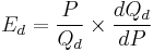
In other words, it is equal to the absolute value of the first derivative of quantity with respect to price (dQd/dP) multiplied by the point's price (P) divided by its quantity (Qd).[15]
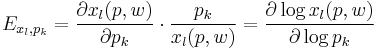
In terms of partial-differential calculus, point-price elasticity of demand can be defined as follows:[16] let  be the demand of goods
 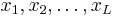 as a function of parameters price and wealth, and let
  be the demand for good
  . The elasticity of demand for good with respect to price
  is
is
However, the point-price elasticity can be computed only if the formula for the demand function,  , is known so its derivative with respect to price,
  , can be determined.
Arc elasticity
A second solution to the asymmetry problem of having a PED dependent on which of the two given points on a demand curve is chosen as the "original" point and which as the "new" one is to compute the percentage change in P and Q relative to the average of the two prices and the average of the two quantities, rather than just the change relative to one point or the other. Loosely speaking, this gives an "average" elasticity for the section of the actual demand curve—i.e., the arc of the curve—between the two points. As a result, this measure is known as the arc elasticity, in this case with respect to the price of the good. The arc elasticity is defined mathematically as:[13][17][18]
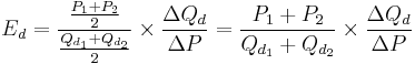
This method for computing the price elasticity is also known as the "midpoints formula", because the average price and average quantity are the coordinates of the midpoint of the straight line between the two given points.[12][18] However, because this formula implicitly assumes the section of the demand curve between those points is linear, the greater the curvature of the actual demand curve is over that range, the worse this approximation of its elasticity will be.[17][19]
History
Together with the concept of an economic "elasticity" coefficient, Alfred Marshall is credited with defining PED ("elasticity of demand") in his book Principles of Economics, published in 1890.[20] He described it thus: "And we may say generally:— the elasticity (or responsiveness) of demand in a market is great or small according as the amount demanded increases much or little for a given fall in price, and diminishes much or little for a given rise in price".[21] He reasons this since "the only universal law as to a person's desire for a commodity is that it diminishes... but this diminution may be slow or rapid. If it is slow... a small fall in price will cause a comparatively large increase in his purchases. But if it is rapid, a small fall in price will cause only a very small increase in his purchases. In the former case... the elasticity of his wants, we may say, is great. In the latter case... the elasticity of his demand is small."[22] Mathematically, the Marshallian PED was based on a point-price definition, using differential calculus to calculate elasticities.[23]
Determinants
The overriding factor in determining PED is the willingness and ability of consumers after a price change to postpone immediate consumption decisions concerning the good and to search for substitutes ("wait and look").[24] A number of factors can thus affect the elasticity of demand for a good:[25]
- Availability of substitute goods: the more and closer the substitutes available, the higher the elasticity is likely to be, as people can easily switch from one good to another if an even minor price change is made;[25][26][27] There is a strong substitution effect.[28] If no close substitutes are available the substitution of effect will be small and the demand inelastic.[28]
- Breadth of definition of a good: the broader the definition of a good (or service), the lower the elasticity. For example, Company X's fish and chips would tend to have a relatively high elasticity of demand if a significant number of substitutes are available, whereas food in general would have an extremely low elasticity of demand because no substitutes exist.[29]
- Percentage of income: the higher the percentage of the consumer's income that the product's price represents, the higher the elasticity tends to be, as people will pay more attention when purchasing the good because of its cost;[25][26] The income effect is substantial.[30] When the goods represent only a negligible portion of the budget the income effect will be insignificant and demand inelastic,[30]
- Necessity: the more necessary a good is, the lower the elasticity, as people will attempt to buy it no matter the price, such as the case of insulin for those that need it.[10][26]
- Duration: for most goods, the longer a price change holds, the higher the elasticity is likely to be, as more and more consumers find they have the time and inclination to search for substitutes.[25][27] When fuel prices increase suddenly, for instance, consumers may still fill up their empty tanks in the short run, but when prices remain high over several years, more consumers will reduce their demand for fuel by switching to carpooling or public transportation, investing in vehicles with greater fuel economy or taking other measures.[26] This does not hold for consumer durables such as the cars themselves, however; eventually, it may become necessary for consumers to replace their present cars, so one would expect demand to be less elastic.[26]
- Brand loyalty: an attachment to a certain brand—either out of tradition or because of proprietary barriers—can override sensitivity to price changes, resulting in more inelastic demand.[29][31]
- Who pays: where the purchaser does not directly pay for the good they consume, such as with corporate expense accounts, demand is likely to be more inelastic.[31]
Interpreting values of price elasticity coefficients
Elasticities of demand are interpreted as follows:[10]
| Value | Descriptive Terms |
|---|---|
| Ed = 0 | Perfectly inelastic demand |
| - 1 < Ed < 0 | Inelastic or relatively inelastic demand |
| Ed = - 1 | Unit elastic, unit elasticity, unitary elasticity, or unitarily elastic demand |
| - ∞ < Ed < - 1 | Elastic or relatively elastic demand |
| Ed = - ∞ | Perfectly elastic demand |
A decrease in the price of a good normally results in an increase in the quantity demanded by consumers because of the law of demand, and conversely, quantity demanded decreases when price rises. As summarized in the table above, the PED for a good or service is referred to by different descriptive terms depending on whether the elasticity coefficient is greater than, equal to, or less than −1. That is, the demand for a good is called:
- relatively inelastic when the percentage change in quantity demanded is less than the percentage change in price (so that Ed > - 1);
- unit elastic, unit elasticity, unitary elasticity, or unitarily elastic demand when the percentage change in quantity demanded is equal to the percentage change in price (so that Ed = - 1); and
- relatively elastic when the percentage change in quantity demanded is greater than the percentage change in price (so that Ed < - 1).[10]
As the two accompanying diagrams show, perfectly elastic demand is represented graphically as a horizontal line, and perfectly inelastic demand as a vertical line. These are the only cases in which the PED and the slope of the demand curve (∆P/∆Q) are both constant, as well as the only cases in which the PED is determined solely by the slope of the demand curve (or more precisely, by the inverse of that slope).[10]
Effect on total revenue
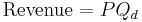
A firm considering a price change must know what effect the change in price will have on total revenue. Revenue is simply the product of unit price times quantity:
Generally any change in price will have two effects:[32]
- the price effect : For inelastic goods, an increase in unit price will tend to increase revenue, while a decrease in price will tend to decrease revenue. (The effect is reversed for elastic goods.)
- the quantity effect : an increase in unit price will tend to lead to fewer units sold, while a decrease in unit price will tend to lead to more units sold.
For inelastic goods, because of the inverse nature of the relationship between price and quantity demanded (i.e., the law of demand), the two effects affect total revenue in opposite directions. But in determining whether to increase or decrease prices, a firm needs to know what the net effect will be. Elasticity provides the answer: The percentage change in total revenue is approximately equal to the percentage change in quantity demanded plus the percentage change in price. (One change will be positive, the other negative.)[33] The percentage change in quantity is related to the percentage change in price by elasticity: hence the percentage change in revenue can be calculated by knowing the elasticity and the percentage change in price alone.
As a result, the relationship between PED and total revenue can be described for any good:[34][35]
- When the price elasticity of demand for a good is perfectly inelastic (Ed = 0), changes in the price do not affect the quantity demanded for the good; raising prices will cause total revenue to increase.
- When the price elasticity of demand for a good is relatively inelastic (-1 < Ed < 0), the percentage change in quantity demanded is smaller than that in price. Hence, when the price is raised, the total revenue rises, and vice versa.
- When the price elasticity of demand for a good is unit (or unitary) elastic (Ed = -1), the percentage change in quantity is equal to that in price, so a change in price will not affect total revenue.
- When the price elasticity of demand for a good is relatively elastic ( -∞ < Ed < -1), the percentage change in quantity demanded is greater than that in price. Hence, when the price is raised, the total revenue falls, and vice versa.
- When the price elasticity of demand for a good is perfectly elastic (Ed is − ∞), any increase in the price, no matter how small, will cause demand for the good to drop to zero. Hence, when the price is raised, the total revenue falls to zero.
Hence, as the accompanying diagram shows, total revenue is maximized at the combination of price and quantity demanded where the elasticity of demand is unitary.[35]
It is important to realize that price-elasticity of demand is not necessarily constant over all price ranges. The linear demand curve in the accompanying diagram illustrates that changes in price also change the elasticity: the price elasticity is different at every point on the curve.
Effect on tax incidence
PEDs, in combination with price elasticity of supply (PES), can be used to assess where the incidence (or "burden") of a per-unit tax is falling or to predict where it will fall if the tax is imposed. For example, when demand is perfectly inelastic, by definition consumers have no alternative to purchasing the good or service if the price increases, so the quantity demanded would remain constant. Hence, suppliers can increase the price by the full amount of the tax, and the consumer would end up paying the entirety. In the opposite case, when demand is perfectly elastic, by definition consumers have an infinite ability to switch to alternatives if the price increases, so they would stop buying the good or service in question completely—quantity demanded would fall to zero. As a result, firms cannot pass on any part of the tax by raising prices, so they would be forced to pay all of it themselves.[36]
In practice, demand is likely to be only relatively elastic or relatively inelastic, that is, somewhere between the extreme cases of perfect elasticity or inelasticity. More generally, then, the higher the elasticity of demand compared to PES, the heavier the burden on producers; conversely, the more inelastic the demand compared to PES, the heavier the burden on consumers. The general principle is that the party (i.e., consumers or producers) that has fewer opportunities to avoid the tax by switching to alternatives will bear the greater proportion of the tax burden.[36]
Selected price elasticities
Various research methods are used to calculate price elasticities in real life, including analysis of historic sales data, both public and private, and use of present-day surveys of customers' preferences to build up test markets capable of modelling such changes. Alternatively, conjoint analysis (a ranking of users' preferences which can then be statistically analysed) may be used.[37]
Though PEDs for most demand schedules vary depending on price, they can be modeled assuming constant elasticity.[38] Using this method, the PEDs for various goods—intended to act as examples of the theory described above—are as follows. For suggestions on why these goods and services may have the PED shown, see the above section on determinants of price elasticity.
|
See also
- Arc elasticity
- Cross elasticity of demand
- Income elasticity of demand
- Price elasticity of supply
- Supply and demand
- Yield elasticity of bond value
Notes
- ^ a b Png, Ivan (1999). p.57.
- ^ Parkin; Powell; Matthews (2002). pp.74-5.
- ^ a b Gillespie, Andrew (2007). p.43.
- ^ a b Gwartney, James D.; Stroup, Richard L.; Sobel, Russell S. (2008). p.425.
- ^ Gillespie, Andrew (2007). p.57.
- ^ Ruffin; Gregory (1988). p.524.
- ^ Ferguson, C.E. (1972). p.106.
- ^ Ruffin; Gregory (1988). p.520
- ^ McConnell; Brue (1990). p.436.
- ^ a b c d e f g Parkin; Powell; Matthews (2002). p.75.
- ^ McConnell; Brue (1990). p.437
- ^ a b Ruffin; Gregory (1988). pp.518-519.
- ^ a b Ferguson, C.E. (1972). pp.100-101.
- ^ Sloman, John (2006). p.55.
- ^ Wessels, Walter J. (2000). p. 296.
- ^ Mas-Colell; Winston; Green (1995).
- ^ a b Wall, Stuart; Griffiths, Alan (2008). pp.53-54.
- ^ a b McConnell;Brue (1990). pp.434-435.
- ^ Ferguson, C.E. (1972). p.101n.
- ^ Taylor, John (2006). p.93.
- ^ Marshall, Alfred (1890). III.IV.2.
- ^ Marshall, Alfred (1890). III.IV.1.
- ^ Schumpeter, Joseph Alois; Schumpeter, Elizabeth Boody (1994). p. 959.
- ^ Negbennebor (2001).
- ^ a b c d Parkin; Powell; Matthews (2002). pp.77-9.
- ^ a b c d e Walbert, Mark. "Tutorial 4a". http://www.ilstu.edu/~mswalber/ECO240/Tutorials/Tut04/Tutorial04a.html. Retrieved 27 February 2010.
- ^ a b Goodwin, Nelson, Ackerman, & Weisskopf (2009).
- ^ a b Frank (2008) 118.
- ^ a b Gillespie, Andrew (2007). p.48.
- ^ a b Frank (2008) 119.
- ^ a b Png, Ivan (1999). p.62-3.
- ^ Krugman, Wells (2009). p.151.
- ^ Goodwin, Nelson, Ackerman & Weisskopf (2009). p.122.
- ^ Gillespie, Andrew (2002). p.51.
- ^ a b Arnold, Roger (2008). p. 385.
- ^ a b Wall, Stuart; Griffiths, Alan (2008). pp.57-58.
- ^ Png, Ivan (1999). pp.79-80.
- ^ "Constant Elasticity Demand and Supply Curves (Q=A*P^c)". http://wpscms.pearsoncmg.com/aw_perloff_microecon_3/9/2365/605606.cw/index.html. Retrieved 26 April 2010.
- ^ Perloff, J. (2008). p.97.
- ^ Chaloupka, Frank J.; Grossman, Michael; Saffer, Henry (2002); Hogarty and Elzinga (1972) cited by Douglas Greer in Duetsch (1993).
- ^ Pindyck; Rubinfeld (2001). p.381.; Steven Morrison in Duetsch (1993), p. 231.
- ^ Richard T. Rogers in Duetsch (1993), p.6.
- ^ "Demand for gasoline is more price-inelastic than commonly thought". Energy Economics. http://dx.doi.org/10.1016/j.eneco.2011.09.003. Retrieved 11 December 2011.
- ^ a b c Samuelson; Nordhaus (2001).
- ^ Goldman and Grossman (1978) cited in Feldstein (1999), p.99
- ^ Perloff, J. (2008).
- ^ Heilbrun and Gray (1993, p.94) cited in Vogel (2001)
- ^ Goodwin; Nelson; Ackerman; Weissskopf (2009). p.124.
- ^ Brownell, Kelly D.; Farley, Thomas; Willett, Walter C. et al. (2009).
- ^ a b Ayers; Collinge (2003). p.120.
- ^ Barnett and Crandall in Duetsch (1993), p.147
- ^ Krugman and Wells (2009) p.147.
- ^ "Profile of The Canadian Egg Industry". Agriculture and Agri-Food Canada. http://www.agr.gc.ca/poultry/prinde3_eng.htm#sec312. Retrieved 9 September 2010.
- ^ Cleasby, R. C. G.; Ortmann, G. F. (1991). "Demand Analysis of Eggs in South Africa". Agrekon 30 (1): 34–36. doi:10.1080/03031853.1991.9524200.
References
- Arnold, Roger A. (17 December 2008). Economics. Cengage Learning. ISBN 9780324595420. http://books.google.com/books?id=EGeEMRfsrRsC. Retrieved 28 February 2010.
- Ayers; Collinge (2003). Microeconomics. Pearson. ISBN 053653313X.
- Brownell, Kelly D.; Farley, Thomas; Willett, Walter C.; Popkin, Barry M.; Chaloupka, Frank J.; Thompson, Joseph W.; Ludwig, David S. (15 October 2009). "The Public Health and Economic Benefits of Taxing Sugar-Sweetened Beverages". New England Journal of Medicine 361 (16): 1599–1605. doi:10.1056/NEJMhpr0905723. PMC 3140416. PMID 19759377. http://content.nejm.org/cgi/content/full/NEJMhpr0905723.
- Case, Karl; Fair, Ray (1999). Principles of Economics (5th ed.). Prentice-Hall. ISBN 0-13-961905-4.
- Chaloupka, Frank J.; Grossman, Michael; Saffer, Henry (2002). "The effects of price on alcohol consumption and alcohol-related problems". Alcohol Research and Health.
- Duetsch, Larry L. (1993). Industry Studies. Englewood Cliffs, NJ: Prentice Hall. ISBN 0585019797.
- Feldstein, Paul J. (1999). Health Care Economics (5th ed.). Albany, NY: Delmar Publishers. ISBN 0766806995.
- Ferguson, Charles E. (1972). Microeconomic Theory (3rd ed.). Homewood, Illinois: Richard D. Irwin. ISBN 0256021570.
- Frank, Robert (2008). Microeconomics and Behavior (7th ed.). McGraw-Hill. ISBN 978-007-126349-8.
- Gillespie, Andrew (1 March 2007). Foundations of Economics. Oxford University Press. ISBN 9780199296378. http://books.google.com/books?id=9NoT4gnYvPMC. Retrieved 28 February 2010.
- Goodwin; Nelson; Ackerman; Weisskopf (2009). Microeconomics in Context (2nd ed.). Sharpe. ISBN 061834599X.
- Gwartney, James D.; Stroup, Richard L.; Sobel, Russell S.; David MacPherson (14 January 2008). Economics: Private and Public Choice. Cengage Learning. ISBN 9780324580181. http://books.google.com/books?id=yIbH4R77OtMC. Retrieved 28 February 2010.
- Krugman; Wells (2009). Microeconomics (2nd ed.). Worth. ISBN 978-0-7167-7159-3.
- Landers (February 2008). Estimates of the Price Elasticity of Demand for Casino Gaming and the Potential Effects of Casino Tax Hikes.
- Marshall, Alfred (1920). Principles of Economics. Library of Economics and Liberty. ISBN 0256015473. http://www.econlib.org/library/Marshall/marP12.html. Retrieved 5 March 2010.
- Mas-Colell, Andreu; Winston, Michael D.; Green, Jerry R. (1995). Microeconomic Theory. New York: Oxford University Press. ISBN 1428871519.
- McConnell, Campbell R.; Brue, Stanley L. (1990). Economics: Principles, Problems, and Policies (11th ed.). New York: McGraw-Hill. ISBN 0-07-044967-8.
- Negbennebor (2001). "The Freedom to Choose". Microeconomics. ISBN 1-56226-485-0.
- Parkin, Michael; Powell, Melanie; Matthews, Kent (2002). Economics. Harlow: Addison-Wesley. ISBN 0-273-65813-1.
- Perloff, J. (2008). Microeconomic Theory & Applications with Calculus. Pearson. ISBN 9780321277947.
- Pindyck; Rubinfeld (2001). Microeconomics (5th ed.). Prentice-Hall. ISBN 1405893400.
- Png, Ivan (1999). Managerial Economics. Blackwell. ISBN 9780631225164. http://books.google.co.uk/books?id=SecBA0uR71MC. Retrieved 28 February 2010.
- Ruffin, Roy J.; Gregory, Paul R. (1988). Principles of Economics (3rd ed.). Glenview, Illinois: Scott, Foresman. ISBN 0-673-18871-X.
- Samuelson; Nordhaus (2001). Microeconomics (17th ed.). McGraw-Hill. ISBN 0070579539.
- Schumpeter, Joseph Alois; Schumpeter, Elizabeth Boody (1994). History of economic analysis (12th ed.). Routledge. ISBN 9780415108881. http://books.google.com/books?id=pTylUAXE-toC. Retrieved 5 March 2010.
- Sloman, John (2006). Economics. Financial Times Prentice Hall. ISBN 9780273705123. http://books.google.com/books?id=EotlIrKjdBUC. Retrieved 5 March 2010.
- Taylor, John B. (1 February 2006). Economics. Cengage Learning. ISBN 9780618640850. http://books.google.com/books?id=mZGDHmPHAb4C. Retrieved 5 March 2010.
- Vogel, Harold (2001). Entertainment Industry Economics (5th ed.). Cambridge University Press. ISBN 0521792649.
- Wall, Stuart; Griffiths, Alan (2008). Economics for Business and Management. Financial Times Prentice Hall. ISBN 9780273713678. http://books.google.com/books?id=TrRtUr_Wn2IC. Retrieved 6 March 2010.
- Wessels, Walter J. (1 September 2000). Economics. Barron's Educational Series. ISBN 9780764112744. http://books.google.com/books?id=0hggJhQQQboC. Retrieved 28 February 2010.
External links
- A Lesson on Elasticity in Four Parts, Youtube, Jodi Beggs
- Approx. PED of Various Products (U.S.)
- Approx. PED of Various Home-Consumed Foods (U.K.)